This (long-delayed; sorry, it’s 2020!) final post in my series about Project BirdMap goes into detail about getting the data, processing it, and using it to build the map. Fair warning: from this point, it’s less birdy and more nerdy.
The code for Project BirdMap is available in GitHub: https://github.com/daverodriguez/project-birdmap
Getting data from EOD
In my Building Project BirdMap post, I talked about EOD, the eBird Observation Dataset. The full dataset is over 300 GB in size, but fortunately I could filter down to just what I needed. For my Woodpeckers map, I used the Scientific name filter and browsed down through the bird taxonomy until I found Piciformes (the woodpecker-like order) and finally Picidae (just woodpeckers).
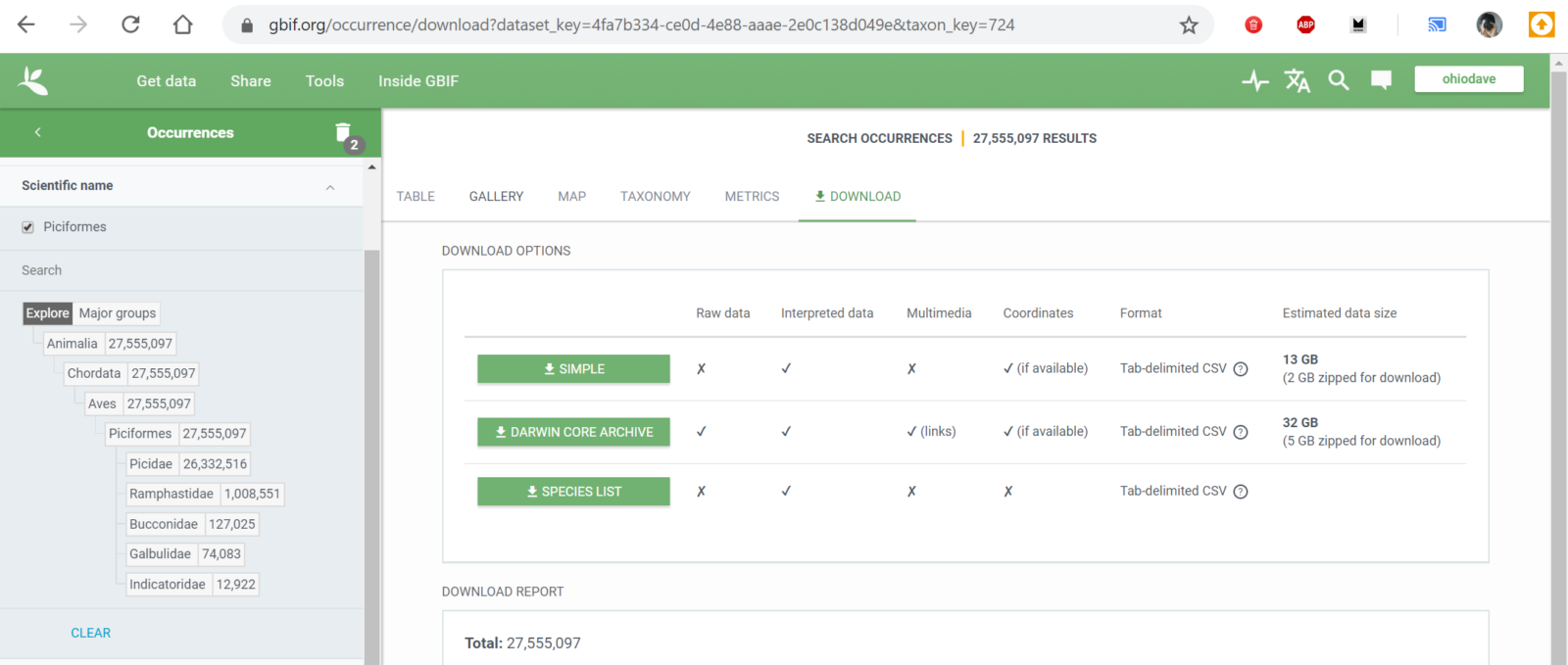
This took the dataset down to a more manageable 13 GB, but to shrink it a little further I filtered on the observation year and pulled only sightings from 2010 to 2020. I figured that if I wanted to know where to travel in 2020 and beyond, historic observations would be less valuable. This left me with a download of 11 GB, or about 23.6 million bird sightings.
A note about bird taxonomy
As I’ve learned and read more about birds, I’ve become semi-familiar with the “taxonomy”, the complete genetic hierarchy of bird families and subfamilies. Once a year, various ornithological unions publish updates to their taxonomies as new research comes in. Species get “split” and “lumped”, renamed, or moved from one family to another. Cornell Labs (the makers of eBird) maintains one such taxonomy and even though you can’t browse the eBird site that way, you can still download the taxonomy datafile. I found that data at https://www.birds.cornell.edu/clementschecklist/download/, and I selected the eBird/Clements Checklist v2019 (CSV flavor).
I used this taxonomy to generate a species list for each family (starting with the woodpeckers) so I could filter my map by species, and later on I found it came in handy sorting out some data anomalies as well.
Working with the data
I’ve used MySQL a lot, but I knew for this project I wouldn’t need to access the database in real-time. For Project BirdMap, the database would be a temporary data store, just something I could query and use to output data files that the map would load. I did a little research and decided on SQLite as a lightweight, self-contained local database.
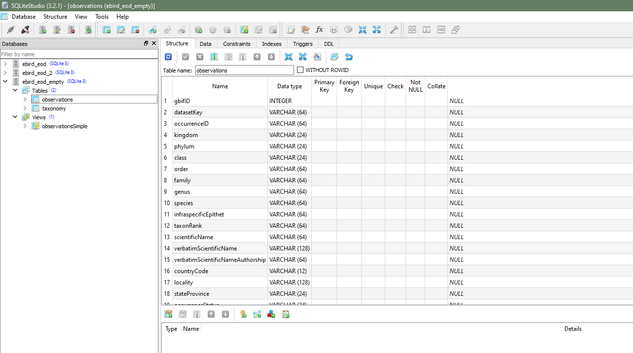
I grabbed SQLiteStudio to use to model my tables, import data, and run queries. I created two tables, observations and taxonomy, and imported the data from my EOD data set and my eBird taxonomy, respectively. For the observations table, I only modeled the first 38 fields, from gbifID up to collectionCode. On import, SQLiteStudio gives me a warning that there are more fields in the data source than the table, but the data import still works just fine.
I did my best to pick datatypes that made sense for each of the fields, but the only ones that really matter are decimalLatitude and decimalLongitude, since my sampling query relies on these being numeric. I picked DOUBLE as the type for each.
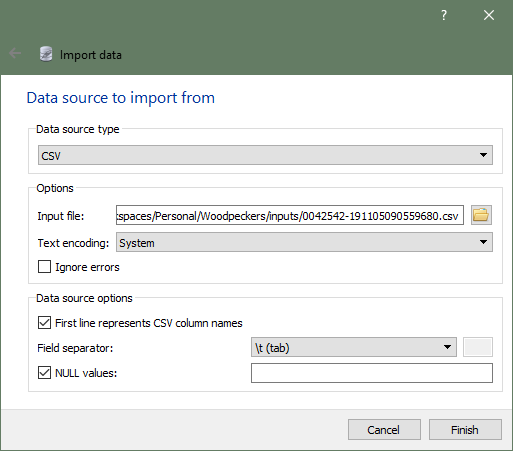
When I was ready to add data, I used SQLiteStudio’s Import into the table. I picked CSV as my Data source type, navigated to my EOD file, and picked my options. A note about EOD data files: even though they have a CSV extension, they use tabs as the separator instead of commas, so you’ll want to set the Field separator property accordingly.
Depending on the size of the data set, import took anywhere from 5 to 30 minutes. As the database got larger, imports got slower and I saw some “Out of memory” errors. I thought SQLite might be loading the database into memory before importing, and even with 24 GB of RAM I was eventually hitting the wall, so if you end up working with multiple large data sets like I did, at some point you might want to split your database into multiple SQLite files.
Also note that deleting data from your tables doesn’t actually make the database smaller. You have to run the VACUUM command to shrink your SQLite file.
I checked a copy of my database into Git, in case you want to use it as a starting point: https://github.com/daverodriguez/project-birdmap/blob/master/data/ebird_eod_empty.db
I left the observations table structure in, but stripped out the data to save space. The taxonomy table and data are intact. In the highly-likely event that Clements publishes an updated taxonomy in the future and you want to reimport it, please note that the taxonomy datafile is a real CSV (with commas as separators) and change your import settings accordingly.
Creating Views
I mentioned that I imported the first 38 fields from EOD, but for sampling I would only use 5 of those: the scientific name, common name, species code (so I could link to the eBird detail page for each bird), and the latitude and longitude. For performance reasons, I created database views with queries like the following:
View: observationsSimple
SELECT verbatimScientificName, PRIMARY_COM_NAME as commonName, SPECIES_CODE as speciesCode, decimalLatitude, decimalLongitude
FROM observations LEFT JOIN taxonomy ON verbatimScientificName = SCI_NAME
Sampling the Data
In the previous post I talked about the GeoJSON file format and the sampling grid I created, dividing the whole world up into latitude/longitude squares. I wrote a Node script to generate the GeoJSON files by querying the database and counting up all the species found in each grid square.
Mapbox (creators of the mapping library I used) also created a Node library to work with SQLite, called node-sqlite3. This made it straightforward to connect to the database and start running queries. I set up my sampling script with some command-line options, including:
- The view name to query
- The min/max latitude and longitude (4 different properties). I added this because sampling grids took a long time to run, and unless I was mapping penguins or certain types of seabirds, most bird families tend to be missing from the highest northern and southern latitudes. My default latitude range was 58° S to 80° N. I default to the full range for longitude, although I could restrict this if I happen to know that some bird family is only present in one hemisphere.
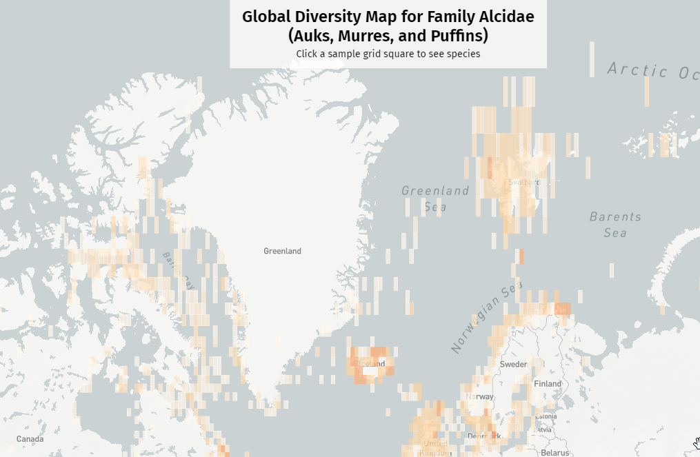
- The sampling grid size, expressed in degrees of latitude and longitude. I’d generally start by running a “quick sample” at a 20×20° grid size, and then a more granular “production pass” at 2×2°, or even 1×1°. One annoying side effect of Mapbox’s Web Mercator map projection is that at extremely high latitudes, the grid squares start to look like vertical rectangles. The further you zoom in, the worse the problem gets, and I don’t know of a solution right now.
My full sampling script is on GitHub (https://github.com/daverodriguez/project-birdmap/blob/master/scripts/sample.js), but here are the highlights:
- The main sampling method loops from min to max longitude, and then min to max latitude. Under default conditions, it starts generating grid squares a spot in the ocean, southeast of New Zealand (and just east of the International Date Line) and works its way east across the world before shifting north and repeating.
- For each grid square, it generates a database query to find all the species found between the lat/lng range, and count the observations of each species:
const query = `SELECT DISTINCT verbatimScientificName, commonName, speciesCode, count(*) AS observationCount FROM ${viewName} WHERE decimalLatitude BETWEEN ${lat} AND ${lat + STEP} AND decimalLongitude BETWEEN ${lng} AND ${lng + STEP} GROUP BY verbatimScientificName ORDER BY observationCount DESC`; - All these queries are queued up using node-sqlite3’s
db.serialize()method, and then run one after another. - As each query finishes, I add the species list and counts to a GeoJSON feature:
const sampleFeature = { type: "Feature", geometry: { type: "Polygon", coordinates: [ [ [lng, lat], [lng + STEP - 0.0001, lat], [lng + STEP - 0.0001, lat + STEP - 0.0001], [lng, lat + STEP - 0.0001], [lng, lat] ] ] }, properties: { lngMin: lng, lngMax: lng + STEP, latMin: lat, latMax: lat + STEP, numSpecies: 0, observedSpecies: [] } }; - At the end, I write the array of GeoJSON features to the output file.
The script-examples readme file has some great working examples of all the options and some real working examples for the sampling script.
Performance Enhancements
On my first run, database performance was awful – each query was taking upwards of a full minute to run. I went back to my database and created an index on the columns I knew I’d be querying to speed things up.
CREATE INDEX species_lat_lng ON observations (
    verbatimScientificName,
    decimalLatitude,
    decimalLongitude
);
It took a few minutes to index the data, but afterwards queries were much snappier. Query time dropped from a minute, to a couple of seconds or less.
Still, at 2 seconds a pop, 12,000 2×2° grid squares could take 6 or 8 hours to run. Early on, I’d run a sample and then find that I needed to tweak something in the data structure. It was irritating to start a multi-hour sample only to find out halfway through that I’d have to stop and run it all over again. To preserve my own sanity, I added three helpful features: skip files, streaming, and runtime metrics.
Skip Files
Waterbirds aside, most birds tend to stay on or near land. One way I found to make the sampling process go faster was to keep a “skip file” of any grid squares that had contained zero species in a previous query. This meant that on subsequent runs, I could skip about 75% of the world and make things go much more quickly.
Streaming and Runtime Metrics
Since production maps took so long to run, I wanted a way to watch them in real time. I updated the script to write partial results to a second “streaming” data file about once a minute. That way, I could watch the map shape up and catch and fix errors without having to wait for the full world map to finish.
I estimated that on a large view, with 2×2° grid squares, one query would take about 2.5 seconds or less to run. That let me calculate approximately how long the full run would take, and report it when running the script. I used the Node humanize-duration library to express the runtime in human-readable terms, e.g. “8 hours, 27 minutes”.
I set a target of trying to update the streaming data file about once per minute, expressed as a “write interval”. At the default 2.5 seconds per second, that works out to one write every 24 grid squares. With every write, I measured the elapsed time since the previous write (or the beginning of the run, for the first write) and extrapolated the time remaining. It wasn’t uncommon to see the remaining time quickly drop from 8 hours, to 6 hours, to 4 hours, after a few write cycles.
Building the Map
Last time, I went into some detail about how I created the map using Mapbox GL JS and built a search and filtering inteface using Vue. The full source of that is available on GitHub.
There are a total of 13 bird maps now, all reading different data files. There’s a single, shared app.js file that loads the data, plots the map, and wires up the interface.
I chose Vue as a framework because I didn’t need a build process and tooling to get started. I could just write Vue-compatible markup, load the framework JavaScript from a CDN, and mount and run my app.
At the end of each file is a script block that denotes the normal data file, streaming data file, and taxonomy file that app.js will load and use.
<script>
  dataFile = "data/sample-data-alcidae.json";
  dataFileStreaming = "data/sample-data-alcidae-streaming.json";
  taxonomyFile = "data/taxonomy-alcidae.json";
</script>
<script src="js/app.js"></script>
The data loading and init code is nice and simple simple:
// Loads the data with fetch
getData().then(data => {
// Filters out oddball observations
normalizeData(data.sampleGrids);
// Initializes the Vue interface
initApp(data);
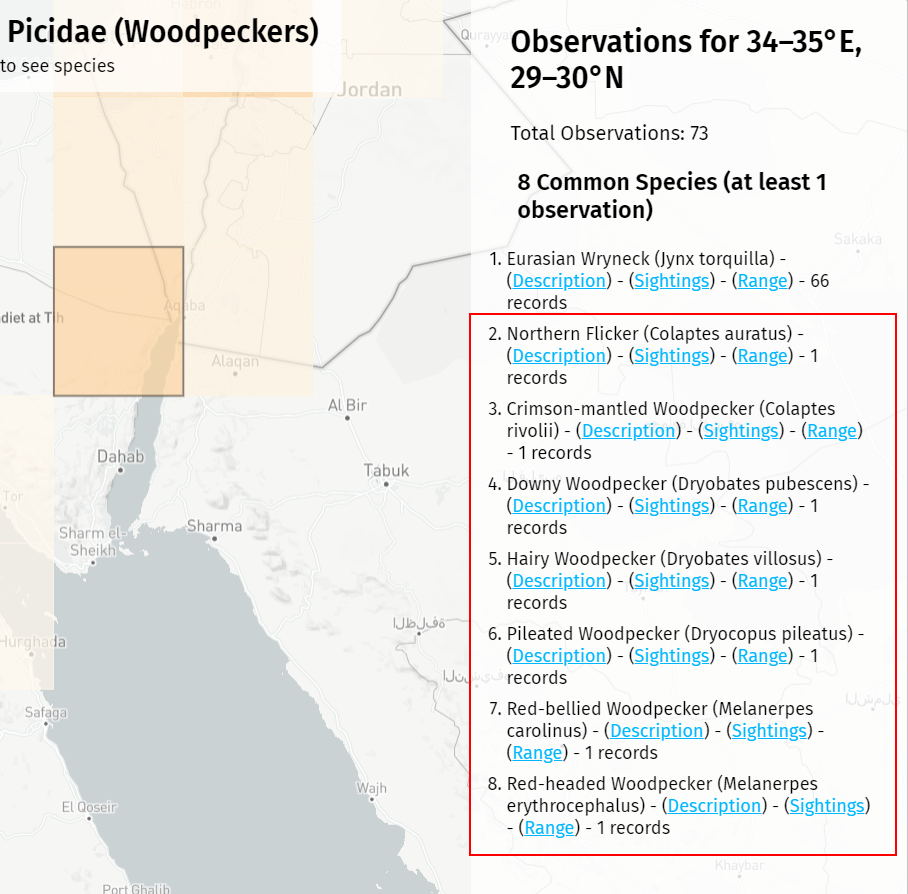
});I added the normalizeData() method after I noticed some odd things in certain grid squares. I found squares where there were 1 or 2 observations (out of tens of thousands) of a species that had no business being in that part of the world. These might have been real vagrant birds, escaped captives, data errors, or intentional lies, but in any case they weren’t helpful. One rogue sighting in 100,000 was not going to give me a clear picture of what I might realistically expect to find in a region. I set a sanity threshold – any species whose total count didn’t make up at least 0.1% of all sightings in a grid square, I sent to a separate “rare” list and omitted from the the map and the observations panel.
In other parts of the world with fewer total observations, rogue species still creep in. In almost every map, I find unexplained North American birds in southern Israel. Again, these could be intentional introductions or escaped birds, but I have a hard time believing people are airlifting Downy Woodpeckers to the Sinai. It feels like bad data to me, and perhaps in time I’ll find another way to filter these out.
I added a couple of optional URL parameters, streaming and debug, that allow me to preview the map while the sample script is still running (by loading the sample-data-streaming.json file) and to debug issues by showing empty sample blocks that are normally hidden.
Adding More Families
Once I had created the Woodpeckers map, I wanted to repeat the process for other kinds of birds. Fortunately, this was pretty easy. I started by downloading more data sets from EOD, filtered by other bird families (and in one case, a whole order – the Strigiformes, owls and barn owls). I imported them into my SQLite database with a different table name, e.g. observations_corvidae for the crows, jays, and magpies. I had to duplicate the index I created for performance reasons as well.
Next I duplicated the view that I’d created to only query the few fields that mattered and named it something like observationsSimpleCorvidae. After a few quick modifications to the sample script, I could then run the sampling process on a whole new data set and start to generate GeoJSON files for a different bird family.
node sample --db="ebird_eod_2.db" --viewname="observationsSimpleCorvidae" --outfile="sample-data-corvidae.json" --step="2" --reset="true"The finches that weren’t finches
Besides the out-of-place birds I mentioned above, I found one other major data anomaly. When I was running the map for Fringillidae – the finches and euphonias, I was partway up South America when I started seeing birds that made me scratch my head.
Leistes loyca, the Long-tailed Meadowlark, is a large and striking bird with a black back, a white supercilium, and a bright-red belly. Very cool, but clearly not a finch. It’s an icterid, related to our North American meadowlarks, as well as red-winged blackbirds, grackles, and orioles. I went into the database and found thousands of observations for 4 different Leistes species, all classified as members of Fringillidae.
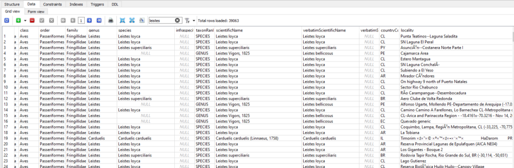
Sometimes birds do get moved around between families, but I think this is just another data bug. With hundreds of millions of records, errors are bound to occur. I filed an issue in the EOD GitHub and started figuring out how to work around the problem. Luckily, it wasn’t too hard. I already had the separate taxonomy table, and there, Leistes was classified correctly as an icterid. I modified my view query a little bit to filter out anything that the taxonomy didn’t identify as belonging to Fringillidae.
SELECT verbatimScientificName, PRIMARY_COM_NAME AS commonName, SPECIES_CODE AS speciesCode, decimalLatitude, decimalLongitude
FROM observations_fringillidae LEFT JOIN taxonomy ON verbatimScientificName = SCI_NAME
where taxonomy.FAMILY = 'Fringillidae (Finches, Euphonias, and Allies)'
Later enhancements
In December 2020 as I’ve added four new bird maps, I’ve added a few new features as well.
Adaptive chloropleth
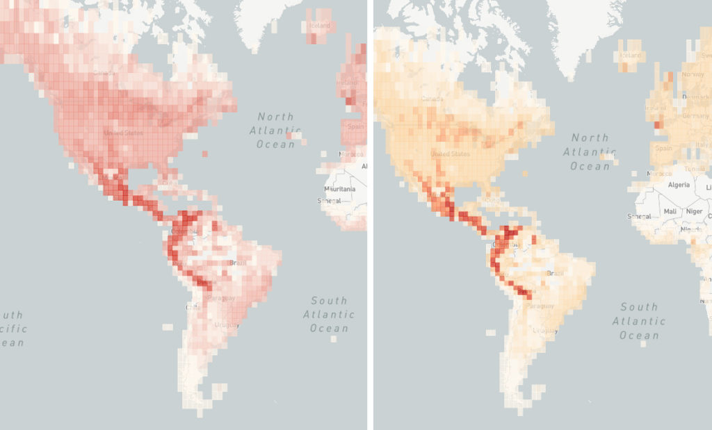
After 13 maps, I wanted to take a look at my original chloropleth color scale. The original scale was based on woodpecker diversity, with an uneven color scale from white to dark red on a scale from 1 to 40 species per grid square. Extending that to other families made some maps unnecessarily muddy, with large chunks of the map all the same color, and it was sometimes hard to pick out regional hotspots.
I decided that the upper bound of the color scale should be flexible. I added a method to the app to go through the data and find the largest number of species in any one square. I defined that as my top-end (the deepest red color) and scaled the remaining colors between 1 and the maximum. Now, regardless of the number of species, every map will have a full range of light and dark areas representing squares with less and more diversity.
I want to give credit to ColorBrewer 2.0, a site that allowed me to generate a custom chloropleth color scheme to help make the visualization more vivid and clear.
Filtering out extinct and unobserved species
A side benefit of checking all the grid data and counting species was that I could check to see if the species in my taxonomy file were actually represented anywhere in the map. The eBird taxonomy includes extinct species, and species that are so rare that there are no recent observations anywhere in the world. It was frustrating to click a species name and see the map go completely blank, and then pull up the eBird description to see that it was now extinct. After this update, only species that occur at least once on the map appear in the list.
Map range zooming
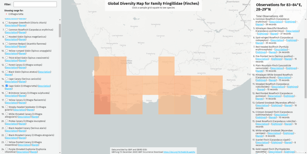
I programmed the original map to be filterable: to show the range of one species, or the range where several species overlap. In the December 2020 revision, I updated the map so when it filters, it also zooms in on filtered range. Now, when you click on the Cape Siskin, a cute little yellow-and-brown finch, the map will zoom you to the corner of southernmost Africa where it can be found. This makes it easier to pinpoint species with a very limited range.
In conclusion, I’ve learned a ton building Project BirdMap, both about birds and about the various technologies that I’ve described here. I’m still having a lot of fun with the project and I have lots more planned for the new year!